from matplotlib import pyplot as plt
import numpy as npSVD Image Compression
Compressing files is a key computational procedure. One approach to image compression is Singular Value Decomposition, where a matrix is broken down into its nonzero (singular) values and two orthagonal matrices. By choosing only a subset of the singular values from which to reconstruct the image, we can achieve significant reductions in image size while retaining a high degree of clarity. In this blog, I explore the process of breaking down and reconstructing an image using different subsets of an image’s singular values.
Let’s begin by reading in an image and converting it to grayscale. I chose the famous Earthrise image from the Apollo 8 mission.
import PIL
import urllib

def read_image(url):
    return np.array(PIL.Image.open(urllib.request.urlopen(url)))
url = 'https://www.nasa.gov/sites/default/files/thumbnails/image/apollo08_earthrise.jpg'
img = read_image(url)code
fig, axarr = plt.subplots(1, 2, figsize = (10, 5))

def to_greyscale(im):
    return 1 - np.dot(im[...,:3], [0.2989, 0.5870, 0.1140])

grey_img = to_greyscale(img)

axarr[0].imshow(img)
axarr[0].axis("off")
axarr[0].set(title = "original")

axarr[1].imshow(grey_img, cmap = "Greys")
axarr[1].axis("off")
axarr[1].set(title = "greyscale")
[Text(0.5, 1.0, 'greyscale')]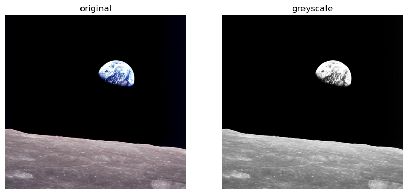
grey_img.shape(2190, 2280)Calculate SVD of gray image
We can calculate the SVD of the gray image using the formula \(A = UDV^T\) where U and V are orthoganal matrices and D has nonzero entries only on its diagonal. The np.linalg.svd function gives us the values needed to reconstruct D.
U, sigma, V = np.linalg.svd(grey_img)
D = np.zeros_like(grey_img,dtype=float) # matrix of zeros of same shape as A
D[:min(grey_img.shape),:min(grey_img.shape)] = np.diag(sigma)        # singular values on the main diagonal
(2190, 2280)Applying this process to a smaller subset of U, D, and V - that is to say, the first k columns of U, the top k values in D, and the first k rows of V - lets us approximate the original image.
Below, the function svd_reconstruct does this for an image and a value k. It first calculates the singular value decomposition of an image, then reconstructs it and returns based on the number of singular values specified by the users.
show it to me
def svd_reconstruct(img,k,compFactor):
    if(compFactor > 0): # if you would rather specify degree of compression than enter a value for k, set compFactor to
                        # a value greater than zero. For example, calling svd_reconstruct(img = img,k = 0, compFactor = 10)
                        # would compress the image to 10% of its original size.

        origSize = img.shape[0] * img.shape[1]
        desiredSize = (origSize/compFactor)
        k = round(desiredSize/(img.shape[0] + img.shape[1] + 1))

    U, sigma, V = np.linalg.svd(img)
    D = np.zeros_like(img,dtype=float) # matrix of zeros of same shape as A
    D[:min(img.shape),:min(img.shape)] = np.diag(sigma) # singular values on the main diagonal

    U_ = U[:,:k] # take a m * k subset of U
    D_ = D[:k, :k] # and the top k values of D
    V_ = V[:k, :] # and an n * k subset of V
    A_ = U_ @ D_ @ V_ # and multiply them all together to reconstruct the image!

    return(A_)

reconImg = svd_reconstruct(grey_img,30,0) # Image reconstructed with top 30 singular values
plt.imshow(reconImg,cmap = 'Greys')
plt.axis('off')
(-0.5, 2279.5, 2189.5, -0.5)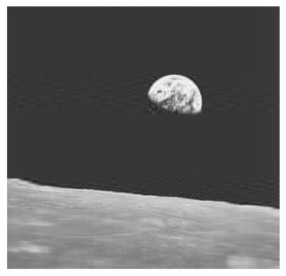
How much compression does this achieve?
Logically, an uncompressed image’s size is proportional to the number of pixels. So, \(m \cdot n\). for an \(m\) x \(n\) image
For compressed images, the size is directly proportional to k. We can calculate it using the formula \(k(m + n + 1)\). We get this because we multiply k*m values in U by a k*k matrix in D, although it actually only has a size of k since values are only along the diagonal, and a k*n subset of V. This gives \(k*m + k * k*n = k(m + 1 + n)\).
Below, we define a function to calculate the compression ratio: \(\frac{originalSize}{compressedSize}\) and the percent storage \(\frac{compressedSize}{originalSize} \cdot 100\)
click here to
def compression(img,k):
    m = img.shape[0]
    n = img.shape[1]
    origSize = m * n
    compressedSize = k * (m + n + 1)
    percentStorage = compressedSize/origSize * 100
    compressionRatio = origSize/compressedSize

    return percentStorage,compressionRatio
Reconstructing images based on compression factor instead of k values
In our svd_reconstruct function, we can specify a degree of compression instead of the number of singular values to use, and use the math shown above to calculate the corresponding k values and generate a reconstruction.
reconImg2 = svd_reconstruct(grey_img,0,20)
reconImg3 = svd_reconstruct(grey_img,0,4)
fig, axarr = plt.subplots(1, 2, figsize = (7, 3))
axarr[0].imshow(reconImg2,cmap = 'Greys')
axarr[0].set(title = 'reconstructed image, storage = 5%')
axarr[0].axis('off')
axarr[1].imshow(reconImg3,cmap = 'Greys')
axarr[1].set(title = 'reconstructed image, storage = 25%')
axarr[1].axis('off')
(-0.5, 2279.5, 2189.5, -0.5)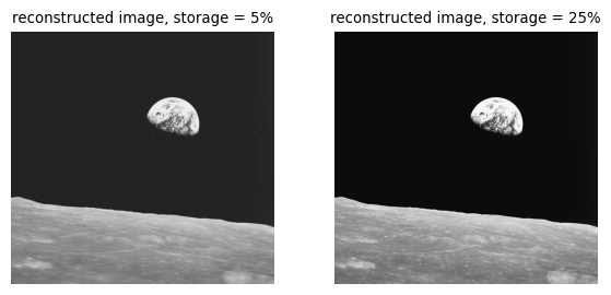
Comparing original to reconstructed images
Below, we show the original image next to an image reconstructed using 30 singular values.
Clearly both show the same thing, but the reconstruction is much less vibrant and is more pixelated.
import math as math
def compare_images(A, A_,k):
    plt.rcParams.update({'font.size': 8})

    fig, axarr = plt.subplots(1, 2, figsize = (7, 3))

    axarr[0].imshow(A, cmap = "Greys")
    axarr[0].axis("off")
    axarr[0].set(title = "original image")

    axarr[1].imshow(A_, cmap = "Greys")
    axarr[1].axis("off")
    axarr[1].set(title = f"reconstructed image, percent storage = {round(compression(grey_img,k)[0],2)}%")

compare_images(grey_img, reconImg,30)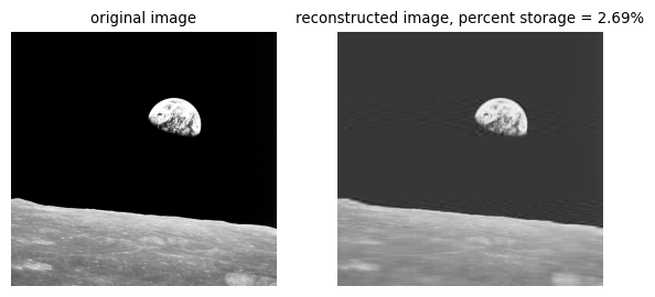
Let’s vizualise the increase in clarity as we use more singular values. The function experiment makes 8 reconstructions using a range of singular values 5-40. By 40 components, we are getting quite close to an accurate representation of the original, though we aren’t quite there yet.
def experiment(img):
    plt.rcParams.update({'font.size': 12})
    imgArr = []
    for i in range(8):
        reconstructed = svd_reconstruct(img, (i + 1) * 5)
        imgArr.append(reconstructed)

    fig, axarr = plt.subplots(2, 4, figsize = (25,15))
    i = 0
    for ax in axarr.ravel():
        ax.imshow(imgArr[i],cmap = 'Greys')
        ax.axis("off")
        ax.set(title = f"{(i+1) * 5} components, \nstorage = {round(compression(grey_img,(i + 1) * 5)[0],2)}%")
        i += 1
experiment(grey_img)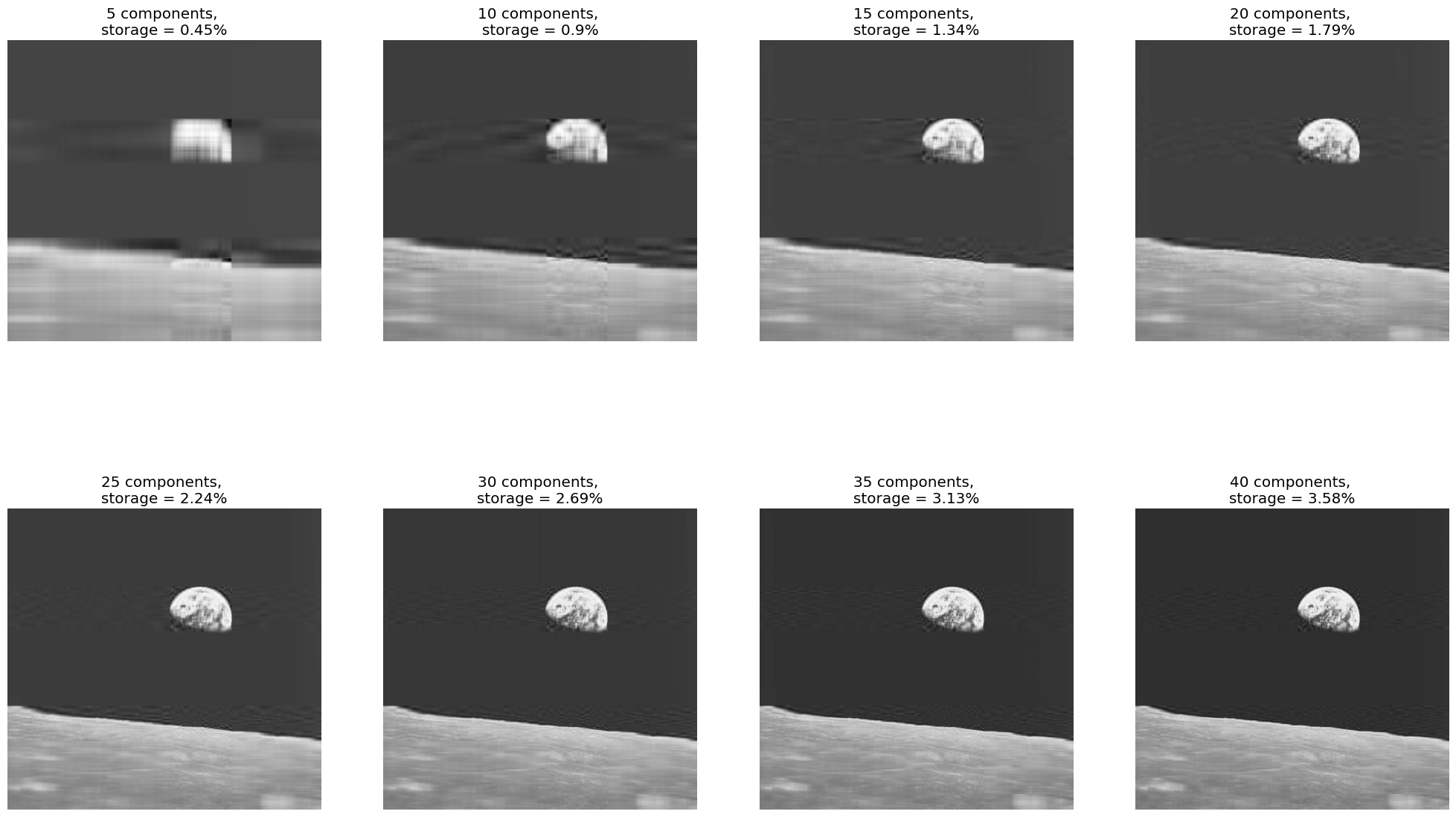
Let’s run a similar experiment, but this time increasing the number of singular values exponentially, starting with 10, to see how the reconstruction looks with a larger number of singular values.
We can see that by the time we hit 100 components, we are really close, and by the time we hit 1000, we are basically at the original, although file size isn’t much smaller than the original by that point.
def experiment2(img):
    plt.rcParams.update({'font.size': 12})
    imgArr = []
    for i in range(3):
        reconstructed = svd_reconstruct(img, 10 ** (i+1),0)
        imgArr.append(reconstructed)

    fig, axarr = plt.subplots(1, 3, figsize = (25,15))
    i = 0
    for ax in axarr.ravel():
        ax.imshow(imgArr[i],cmap = 'Greys')
        ax.axis("off")
        ax.set(title = f"{10 ** (i+1)} components, \nstorage = {round(compression(grey_img,10 ** (i + 1) )[0],2)}%")
        i += 1
    plt.tight_layout()

experiment2(grey_img)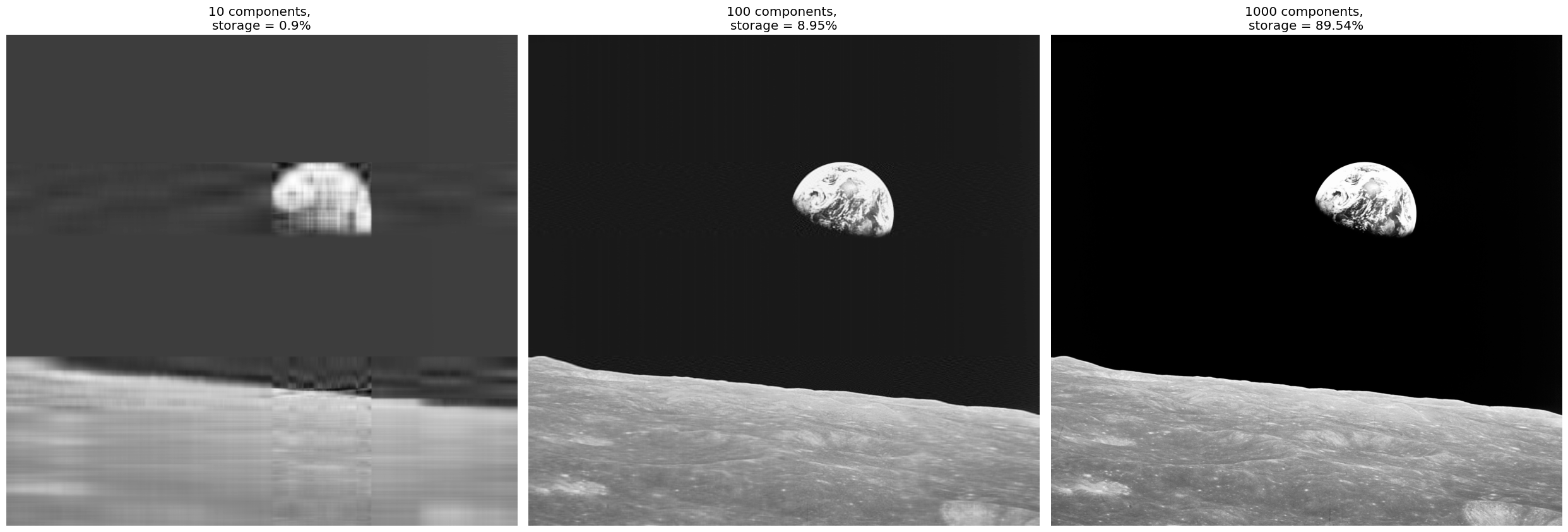
I think taken on their own it’s hard to see the difference between the original and the reconstructions as they get better and better. The reconstruction from 40 singular values, for instance, appears quite clear. But the biggest difference is the intensity of the color as well as some detail on the moon’s surface. It’s really clear when you set reconstructions side by side with the original. Below is a reconstruction with 60 singular values where the difference in clarity to the original image is readily apparent.
recon60 = svd_reconstruct(grey_img,60,0)

compare_images(grey_img, recon60,60)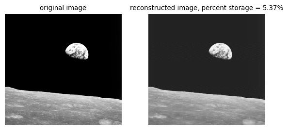
Still, while this reconstruction doesn’t perfectly match the original, it is an excellent approximation and uses only about 5% of the storage space taken by the original image. This is a testament to the power of the SVD process to reduce the size of images.
Recap
The experiments above show the power of SVD image reconstruction. For a given image, the svd_reconstruct function can accept either k, the number of singular values to use, or compFactor, the compression factor we want to achieve, and generate a reconstruction of the original image. Clearly, there are some exciting applications of this process, and it is capable of reproducing a fairly accurate representation of the original image while maintaining a high degree of clarity.